GIS data preparation
Once all necessary layers have been succesfully acquired, the user would need to prepare the datasets for their input into the OnSSET model. This requires the creation of a .csv file. There are four steps that need to be undertaken to process the GIS data so that it can be used for an OnSSET analysis.
Step 1. Proper data types and coordinate system
In this first step the user would need to secure all the datasets. Before starting the analysis make sure that all datasets are in the World Geodetic Datum 1984 (WGS84) / EPSG:4326 coordinate system. You can check the coordinate system of your layers by importing them into QGIS and then right-clicking on them and open the Properties window. In the Properties window go to the Information tab, here the coordinate system used is listed under CRS for both rasters and vectors.
Step 2. Layer projection
In this step the user would need to determine the projection system he/she wish to use. Projection systems always distort the datasets and the system chosen should be one that minimizes this distortion. Do not manually project the datasets yourself (the Jupyter Notebook presented below does this for you). However, it is good to have an idea of which system to use before starting to work with the datasets. Here follows a few important key aspects:
Projection is the systematic transformation of the latitude and longitude of a location into a pair of two dimensional coordinates or else the position of this location on a plane (flat) surface. You will need to select a coordinate system that is measured in meters and appropriate for you region of interest. You can browse coordinate systems at EPSG.io. Search for your country or region, check that the Unit is meters and note down the epsg code.
Step 3. Generate the OnSSET input file
Here, the goal is to take all of the GIS layers that have been collected, and extract the neccessary information to each settlement, which will be saved in a csv-file to be used for running scenarios in the next step.
First, you need to download the codes from here (click on Code and Download zip or clone the repository using Git).
To launch the Jupyter Notebook, open Anaconda Prompt and run the following commands:
cd PATH
conda activate onsset_env
jupyter notebook
Replace PATH with the location on your computer where you downloaded and extracted
the folder containing the OnSSET GIS Extraction codes.
This will open Jupyter in your browser. Note that everything is still running locally; the browser is simply used as the interface.
Open the Notebook
Click on the notebook called csv_file_preparation_stepBystep_code.ipynb
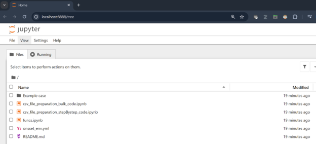
Opening the GIS extraction notebook.
Running Cells
Click on the Run button to run the selected cell (highlighted in blue).
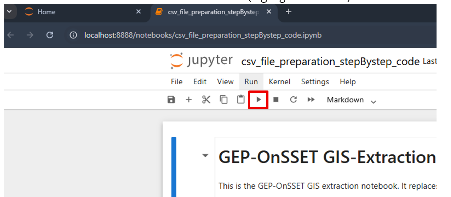
Running a selected cell in Jupyter Notebook.
Importing Packages
The first cell imports the necessary packages and scripts.
If you receive an error message here, it typically means:
Something went wrong with the installation, or
The environment was not activated before launching the notebook.
While a cell is executing, a * appears on the left side of the cell.
Once execution finishes, it is replaced by a number (for example [1]).
Cells containing only text will not show a star or a number.
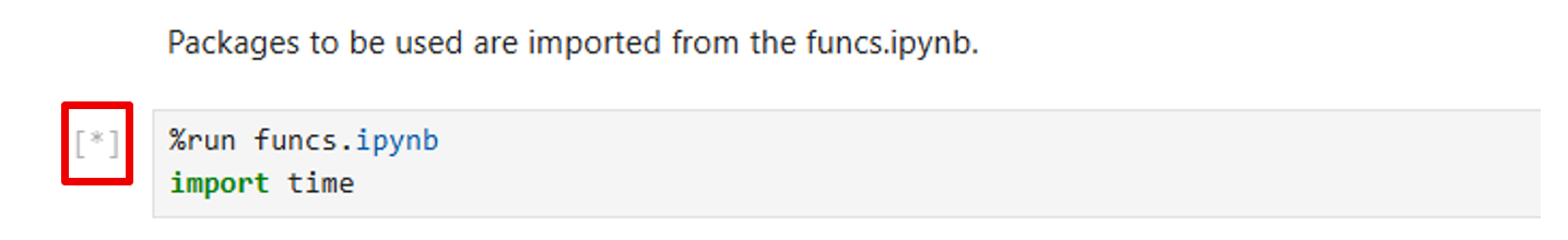
Importing required packages.
Define Coordinate System
In the next cell, define the coordinate system.
You can keep the default or change to the one identified in step 2 (sometimes not all coordinate systems work, so it is suggested to run first with the generic 3395 and then run again with the area-specific one):
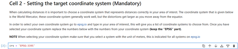
Selecting the coordinate system.
Run the cell to proceed.
Select Output Folder
In the following cell, create or select an empty folder where the results will be saved.
When you run the cell, a pop-up window will appear asking you to select the folder.
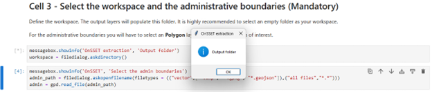
Selecting the output folder.
Selecting Input Datasets
Next, you will select the required GIS datasets.
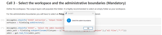
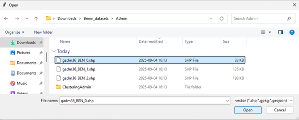
Administrative Boundaries
Select the administrative boundaries layer:
Population Clusters
Select the population clusters layer:
E.g. Benin_datasets > Clusters > Benin.shp
After selecting the file, another pop-up will appear asking you to select the population column.
Choose:
Population
Dataset Selection by Cell
Continue running the cells and select the datasets according to the list below.
If a dataset is not available in the training exercise, simply click Cancel.
Cell 5
E.g. Benin_datasets > Solar > GHI.tif
Cell 6
E.g. Benin_datasets > Traveltime > Traveltime.tif
Cell 7
E.g. Benin_datasets > windvel > windvel.tif
Cell 8
E.g. Benin_datasets > NightLights > NightLights.tif
Cell 9
E.g. Benin_datasets > CustomDemand > CustomizedDemand2.tif
Cell 10
No selection required.
Cell 11
E.g. Benin_datasets > Substations > substations.shp
Cell 12
E.g. Benin_datasets > HV > Existing.shp
Cell 13
E.g. Benin_datasets > HV > Planned.shp
Cell 14
E.g. Benin_datasets > MV > Existing.shp
Cell 15
E.g. Benin_datasets > MV > Planned.shp
Cell 16
E.g. Benin_datasets > Roads > roads.shp
Cell 17
E.g. if not available — click **Cancel**.
Cell 18
E.g. Benin_datasets > Hydro > hydro_points.shp
When prompted, select:
PowerMWMW
Cell 19
E.g. if not available — click **Cancel**.
Cell 20
E.g. Benin_datasets > Admin > GADM36_BEN_1.shp
When prompted, select:
NAME_1 (or other based on your dataset)
Exporting the Results
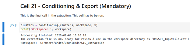
Cell 21
This the final step. Running this cell exports the processed data into a CSV file. If everything works correctly you will see the Processing finished message and the file will be saved in the output folder you selected earlier:
Understanding the Output
In the generated CSV file:
Each row represents one settlement.
Each column represents an attribute used in the OnSSET model.
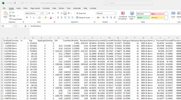
To understand the meaning of each column, refer to the table below or this document which also indicates the expected values in each column.
This CSV file is the final result of the GIS extraction process and will be used in the next exercise to run OnSSET.
GIS country file
The table below shows all the parameters that should be sampled and put into the csv file representing the study area.
Parameter |
Description |
|---|---|
Country |
Name of the country |
Nigthlights |
Maximum light intensity observed in cluster |
Pop |
Population of cluster |
id |
Id of cluster, important when generating maps |
GridCellArea |
Area of each cluster (km2) |
ElecPop |
Population that lives in areas with visible night-time lights |
WindVel |
Wind speed (m/s) |
GHI |
Global Horizontal Irradiation (kWh/m2/year) |
TravelHours |
Distance to the nearest town (hours) |
ResidentialDemandTierCustom |
Indicative residential electricity demand target |
Elevation |
Elevation from sea level (m) |
Slope |
Ground surface slope gradient (degrees) |
LandCover |
Type of land cover as defined by the source data |
CurrentHVLineDist |
Distance to the closest existing HV line (km) |
CurrentMVLineDist |
Distance to the closest existing MV line (km) |
PlannedHVLineDist |
Distance to the closest planned HV line (km) |
PlannedMVLineDist |
Distance to the closest planned MV line (km) |
TransformerDist |
Distance from closest existing transformers (km) |
SubstationDist |
Distance from the existing sub-stations (km) |
RoadDist |
Distance from the existing road network (km) |
HydropowerDist |
Distance from closest identified hydropower potential (km) |
Hydropower |
Closest hydropower technical potential identified |
HydropowerFID |
ID of the nearest hydropower potential |
X_deg |
Longitude |
Y_deg |
Latitude |
IsUrban |
All 0 after extraction, urban/rural split gets assigned in the algorithm |
PerCapitaDemand |
Indicative residential electricity demand target |
HealthDemand |
Indicative electricity demand for health |
EducationDemand |
Indicative electricity demand for educational facilities |
AgriDemand |
Indicative electricity demand for agricultural processes |
ElectrificationOrder |
Indicates order of electrification; retrieved by grid extension algorithm; default =0 |
Conflict |
Indicator of level of conflict (default =0; otherwise option 1-4) |
CommercialDemand |
Indicative electricity demand target for commercial activity |
ResidentialDemandTier1 |
Indicative residential electricity demand target equal to Tier 1 |
ResidentialDemandTier2 |
Indicative residential electricity demand target equal to Tier 2 |
ResidentialDemandTier3 |
Indicative residential electricity demand target equal to Tier 3 |
ResidentialDemandTier4 |
Indicative residential electricity demand target equal to Tier 4 |
ResidentialDemandTier5 |
Indicative residential electricity demand target equal to Tier 5 |
Note
It is very important that the columns in the csv-file are named exactly as they are namned in the Parameter-column in the table above.