GIS data acquisition

Geographic Information Systems

A Geographic Information System (GIS) is an integrated set of hardware and software tools, designed to capture, store, manipulate, analyse, manage, and digitally present spatial (or geographic) data and related attribute information. GIS can relate information from different sources, using two key index variables space (or location) and time. Common GIS data types (models) include:

Spatial Data: Describe the absolute and relative location of geographic features.

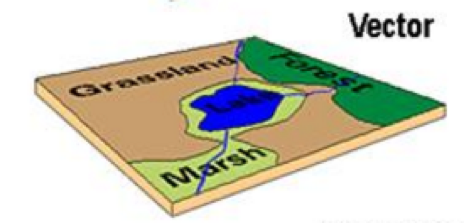
• Vectors

  • Arcs (Polylines): Line segments forming individual linear features

  • Polygons: Areas enclosed by arcs

  • Points: Single coordinate pairs

  

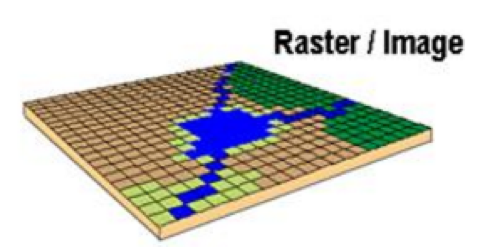
• Rasters

  • Grid-Cells: single column/row positions

  • Cell size: Resolution or else the accuracy of the data

  

Attribute data: Describe characteristics of the spatial features. These characteristics can be quantitative and/or qualitative in nature. Attribute data is often referred to as tabular data.

The selection of a particular data model, vector or raster, is dependent on the source and type of data, as well as the intended use of the data. Certain analytical procedures require raster data while others are better suited to vector data.

GIS data sources

EnergyData.info

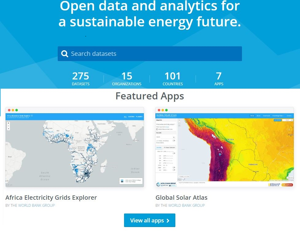
Every day governments, private sector and development aid organizations collect data to inform, prepare and implement policies and investments. Yet, while elaborate reports are made public, the data underpinning the analysis remain locked in a computer out of reach. Because of this, the tremendous value they could bring to public and private actors in data-poor environments is too often lost.

Energydata.info is an open data platform launched recently by The World Bank Group and several partners, trying to change energy data paucity. It has been developed as a public good available to governments, development organizations, non-governmental organizations, academia, civil society and individuals to share data and analytics that can help achieving universal access to modern energy services. The database considers a variety of open, geospatial datasets of various context and granularity. KTH Division of Energy Systems (KTH-dES), formerly known as KTH division of Energy Systems Analysis (KTH-dESA), contributes on a contnuous basis by providing relevant datasets for electrification planning.

Indicative open libraries of GIS data

Over the past few years, KTH dES has been actively involved in the field of geospatial analysis. The following table presents a list of libraries and directories that provide access to open GIS data.

Source	Type	Link
Penn	World per region	http://guides.library.upenn.edu/content.php?pid=324392&sid=2655131
MIT	World per region	http://libguides.mit.edu/c.php?g=176295&p=1161383
EDEnextdata	World per region	https://www.edenextdata.com/?q=content/global-gis-datasets-links-0#Population%20Infrastructure%20Topography%20and%20Administration%20Data
Stanford	World per region	https://library.stanford.edu/research/stanford-geospatial-center/data
GIS Lounge	Finding GIS data	http://www.gislounge.com/data-and-gis-resources/
dragons8mycat	Different countries	https://dragons8mycat.wordpress.com/gis-data-sources/
rtwilson	Different types	http://freegisdata.rtwilson.com/
Planet OSM	Different types	http://planet.osm.org/
Berkeley	Different types	http://gif.berkeley.edu/resources/data_subject.html
Kings College	Different types	http://www.policysupport.org/waterworld
CSRC	Different types	http://rslab.sr.unh.edu/gdatalinks.html
Data Discovery Center	Different types	http://ddc.unh.edu/
Spatial Hydrology	Different types	http://www.spatialhydrology.com/datawarehouse.html
Africa Information Highway	Different types	http://dataportal.opendataforafrica.org/
The Humanitarian Data Exchange	Different types	https://data.humdata.org/

Country specific databases

With geospatial analysis gaining momentun in many research areas, many countries have set up their own geo-databases in an effort to facilitate interdisciplinary research activities under a geospatial context. Here are few examples:

Country	Source
Bolivia	http://geo.gob.bo/#viewer
Brazil	http://www.ibge.gov.br/english/geociencias/default_prod.shtm#REC_NAT
East Timor	http://goleaddog.com/gis-map/asia/timor-leste/
Malawi	http://www.masdap.mw/
Namibia	http://www.uni-koeln.de/sfb389/e/e1/download/atlas_namibia/main_namibia_atlas.html
Nepal	http://geoportal.icimod.org/
Russia	http://gis-lab.info/qa/vmap0-eng.html

GIS data in OnSSET

OnSSET is a GIS-based tool and therefore requires data in a geographical format. In the context of the power sector, necessary data includes those on current and planned infrastructure (electric grid networks, road networks, power plants, industry, public facilities), population characteristics (distribution, location), economic and industrial activity, and local renewable energy flows. The table below lists all layers required for an OnSSET analysis.

#	Dataset	Type	Description
1	Population density & distribution	Raster	Spatial identification and quantification of the current (base year) population. This dataset sets the basis of the ONSSET analysis as it is directly connected with the electricity demand and the assignment of energy access goals.
2	Administrative boundaries	Polygon	Delineates the boundaries of the analysis.
3	Existing HV network (Optional)	Line shapefile	Used to identify and spatially calibrate the currently electrified/non-electrified population. This is layer is optional.
4	Power Substations (Optional)	Point shapefile	Current Substation infrastructure used to identify and spatially calibrate the currently electrified/non-electrified population. It is also used in order to specify grid extension suitability. This is layer is optional.
5	Roads (Optional)	Line shapefile	Current Road infrastructure used to,identify and spatially calibrate the currently electrified/non-electrified population. It is also used in order to specify grid extension suitability. This is layer is optional.
6	Planned HV network (Optional)	Point shapefile	Represents the future plans for the extension of the national electric grid. It also includes extension to current/future substations, power plants, mines and queries. This is layer is optional.
7	Existing MV network (Optional)	Line shapefile	Used to identify and spatially calibrate the currently electrified/non-electrified population. This is layer is optional.
8	Planned MV network (Optional)	Point shapefile	Represents the future plans for the extension of the national electric grid. This is layer is optional.
9	Nighttime lights	Raster	Dataset used to,identify and spatially calibrate the currently electrified/non-electrified population.
10	GHI	Raster	Provide information about the Global Horizontal Irradiation (kWh/m2/year) over an area. This is later used to identify the availability/suitability of Photovoltaic systems.
11	Wind speed	Raster	Provide information about the wind velocity (m/sec) over an area. This is later used to identify the availability/suitability of wind power (using Capacity factors).
12	Hydro power potential (Optional)	Point shapefile	Points showing potential mini/small hydropower potential. Dataset developed by KTH dESA including environmental, social and topological restrictions and provides power availability in each identified point. Other sources can be used but should also provide such information to reassure the proper model function. This is layer is optional.
13	Travel time	Raster	Visualizes spatially the travel time required to reach from any individual cell to the closest town with population more than 50,000 people.
14	Elevation Map	Raster	Filled DEM maps are use in a number of processes in the analysis (Energy potentials, restriction zones, grid extension suitability map etc.).
15	Land Cover	Raster	Land cover maps are use in a number of processes in the analysis (Energy potentials, restriction zones, grid extension suitability map etc.).
16	Service transformers (Optional)	Point shapefile	Current Transformer infrastructure used to identify and spatially calibrate the currently electrified/non-electrified population. This is layer is optional.
17	Custom demand (Optional)	Raster	User defined electricity demand in the end year in each setltement. This is layer is optional.

Note

• Before a model can be built, one must acquire the layers of data outlined above.

• You are recommended to use all the layers listed in the table above, but some of the are optional and can be omited (see table above)

More often than not, each layer must be acquired on its own. The final outcome is a .csv-file conveying all the information necessary to initiate an OnSSET electrification analysis.

GIS basic datasets

Administrative boundaries

Coverage	Type	Resolution	Year	Source	Link
World	shapefile	Counties,provinces, departments, bibhag, bundeslander, daerah istimewa, fivondronana,,krong, landsvæðun, opština, sous-préfectures, counties & thana	2011	GADM	https://gadm.org/
World,(& per country)	shapefile	Countries	2011	DIVA-GIS	http://www.diva-gis.org/Data
Europe	geodatabase/shapefile	Countries, provinces	2013	Eurostat	http://ec.europa.eu/eurostat/web/gisco/geodata/reference-data/administrative-units-statistical-units

Population data

Coverage	Type	Resolution	Year	Source	Link
World	Various	1 arc-second	(depending on country)	HDX	https://data.humdata.org/organization/facebook
World	raster	250 meter and 1 km	1975, 1990, 2000, 2015	Global Human Settlement Layer	https://ghsl.jrc.ec.europa.eu/
Africa, Asia, America	Raster	100 m grid cells	(depending on country)	Worldpop	https://www.worldpop.org/geodata/listing?id=29
World	grid	2.5 arc-minute grid cells	90/95/00	SEDAC	http://sedac.ciesin.columbia.edu/data/set/gpw-v3-population-density/data-download
World	shapefile, raster (grid)	2.5 arc-minute grid cells	2000	UNEP	http://geodata.grid.unep.ch/results.php
Ghana, Haiti, Malawi, South Africa, Sri Lanka	raster (grid)	1 arc-second	2015	CIESIN	https://ciesin.columbia.edu/data/hrsl/
World	Various	Various	2016	dhsprogram	http://spatialdata.dhsprogram.com/home/

Transmission lines data

UK	shapefile	Power transmission lines, underground cables, stations etc.	na	National Grid	http://www2.nationalgrid.com/uk/services/land-and-development/planning-authority/shape-files/
US	raster	100 m grid cells	2015	ArcGIS online	http://www.arcgis.com/home/item.html?id=918e6d9b1cc84d15ba13e911d18a0c5e
World	OSM potential	points or polylines	2015	OSM of various mirrors
World	From Vmap level 0	Power lines and utilities	na	Can be downloaded from:	http://gis-lab.info/qa/vmap0-eng.html

Power plants location data

Coverage	Type	Resolution	Year	Source	Link
World	shapefile (4 levels)	Generators, substations,masts	2009	Vmap level 0	http://gis-lab.info/qa/vmap0-eng.html

Elevation

Coverage	Type	Resolution	Year	Source	Link
World	geoTIFF	30 m spatial resolution	2009	METI Japan, NASA	http://www.jspacesystems.or.jp/ersdac/GDEM/E/2.html
World	geoTIFF	30 m posting, 1x1 degree tiles	2009, 2011	METI Japan, NASA	https://asterweb.jpl.nasa.gov/gdem.asp
World	.bil and/or .tif	15 arcseconds/30arcseconds	various	ISCGM	https://globalmaps.github.io/
World	GeoTIFF	16 arcseconds/30arcseconds	various	NOOA	http://www.ngdc.noaa.gov/mgg/topo/gltiles.html
World	GeoTIFF	17 arcseconds/30arcseconds	various	DGADV	http://www.dgadv.com/dowdem/
World + Arctic areas	GeoTIFF	30 arcseconds	various	WebGIS	http://www.webgis.com/terr_world.html

Travel time to major cities

Coverage	Type	Resolution	Year	Source	Link
World	ESRI grid	30 arc sec	2008 (data from 2000)	Joint Research Center EU	http://forobs.jrc.ec.europa.eu/products/gam/download.php
Africa (sub-Saharan)	csv, ESRI ASCII raster, GeoTIFF	5 arc sec	2010	Harvest Choice	https://dataverse.harvard.edu/dataset.xhtml?persistentId=doi:10.7910/DVN/YKDWJD
World	Raster, GeoTIFF	5 arc sec	2015	Univeristy of Oxford	https://map.ox.ac.uk/explorer/#/explorer

Mining and Quarrying

Coverage	Type	Resolution	Year	Source	Link
USA	Shapefile, csv, KML, KMZ	Active mines and mineral plants in the US	2003	USGS	http://mrdata.usgs.gov/mineplant/
World	Shapefile, dBase, HTML, Tab text,csv, Google earth	points	2012-2013		http://minerals.usgs.gov/minerals/pubs/country/?utm_source=feedburner&utm_medium=feed&utm_campaign=Feed%3A+usgs_mpubs+%28USGS+Minerals+Periodicals%29
					http://mrdata.usgs.gov/mineral-resources/minfac.html
					http://mrdata.usgs.gov/mineral-operations/

Solar

Coverage	Type	Resolution	Year	Source	Link
World	ESRI ASCII GRID, GeoTIFF	250 m	2017	SolarGIS	https://globalsolaratlas.info/

Wind

Coverage	Type	Resolution	Year	Source	Link
World	GeoTIFF	250m	2018	Technological University of Denmark	https://globalwindatlas.info/

Land cover

Coverage	Type	Resolution	Year	Source	Link
World	HDF-EOS	500 m	2001-2018	NASA-MODIS	https://lpdaac.usgs.gov/products/mcd12q1v006/
World	CI Land cover - raster	300 m	time series from 1992 to 2015	ESA	http://maps.elie.ucl.ac.be/CCI/viewer/
World	GeoTiff, Google earth, jpeg,png	1-0.1 degrees	2001-2010	NASA-NEO	http://neo.sci.gsfc.nasa.gov/view.php?datasetId=MCD12C1_T1
World	Raster, csv	0.0028 - 0.0083 degrees	2000, 2005, 2010	ESA-ENVISAT	http://maps.elie.ucl.ac.be/CCI/viewer/index.php
World/Protected areas	Shapefile, KML, csv	na	2014	Protected planet	http://www.protectedplanet.net/
World	various	various	2015	Global Land Cover Facility	http://landcover.org/data/
World	Rasters for: Costal areas, Cultivated areas, Forests, Mountains, Islands, Inland waters etc.	0.00833 degrees	2000	SEDAC	http://sedac.ciesin.columbia.edu/data/set/ma-ecosystems/data-download
World	Raster for croplands	0.0833 degrees	2000	SEDAC	http://sedac.ciesin.columbia.edu/data/set/aglands-croplands-2000/data-download
World	Various Rasters on Land Use	various	1990-2010	Nelson Institute	http://nelson.wisc.edu/sage/data-and-models/datasets.php
World	Soil type	various	na	Worldmap.Harvard	https://worldmap.harvard.edu/data/geonode:DSMW_RdY
World	Various Rasters on Land Use	various	1980-2014	EarthStat	http://www.earthstat.org/data-download/

The model classifies the land cover in order to calculate the grid extension penalties. The default classification values are based on the MODIS dataset found here, where the legend ranges from 1-17 with the values and corresponding land cover type can be seen below. If land cover data is retrieved from other data sources with different classification values they should be reclassified in GIS (using the Reclassify tool in ArcGIS or r.reclass in QGIS) to match those below. Alternatively changes can be made in the Python code instead. If this reclassification is not performed it may lead to an incorrect grid penalty factor or, if the highest values are above 17, an error message while running the code.

Value	Label
1	Evergreen Needleleaf forest
2	Evergreen Broadleaf forest
3	Deciduous Needleleaf forest
4	Deciduous Broadleaf forest
5	Mixed forest
6	Closed shrublands
7	Open shrublands
8	Woody savannas
9	Savannas
10	Grasslands
11	Permanent wetlands
12	Croplands
13	Urban and built-up
14	Cropland/Natural vegetation mosaic
15	Permanent snow and ice
16	Barren
17	Water bodies

Others

Coverage	Type	Resolution	Year	Source	Link
World	Coast Lines, oceans	Physical vectors, ESRI shapefiles, GeoTIFF (1:10, 1:50 and 1:110 m)	2015	Natural Earth	http://www.naturalearthdata.com/downloads/
World	Climate data	30 arc seconds and 2.5/5/10 arc minutes	na	WorldClim	http://www.worldclim.org/
World/USA	Climate change scenarios	various	na	na	https://gisclimatechange.ucar.edu/
World/Australia	Water and Landscape Dynamics	0.05 to 1 degrees	1979-2012	Australian National University	http://www.wenfo.org/wald/data-software/
Open Street Map (OSM) - Osmosis	osm.pbf	depending on mirror source	up to date	NOAA	http://ngdc.noaa.gov/eog/dmsp/downloadV4composites.html
Nighttime lights	Raster file	0.0042 degrees	2012-2020	na	https://eogdata.mines.edu/download_dnb_composites.html
Africa information Highway	various	vectors	various	AfDB	http://dataportal.opendataforafrica.org/
World	Cliamte data	various	various	Oregon State University	http://globalclimatedata.org/

Methodology for Open Street Map data and Osmosis

Note

• Open Street Map (OSM) is a collaborative project that intends to provide free and open access data used in mapping the world. This document aims at describing in brief the methodology used in order to obtain OSM data and transform them in compatible and useful information with the use of Osmosis and QGIS.

• To begin with, bulk download of updated OSM data can be performed through the Planet OSM: http://planet.osm.org/.

• The files can be downloaded as .xml and .pbf format. However, due to the large volume of data there are various mirrors/extracts that provide access to masked data for different regions of the planet. More information can be found here: http://wiki.openstreetmap.org/wiki/Planet.osm#Downloading. In previous cases Geofabrik.de where used successfully (https://download.geofabrik.de/africa.html).

• From Geofabrik, data can be downloaded per region in .pbf format. In the latest version of QGIS it is possible to insert this data directly by simply dragging the file onto the QGIS window. However, since the files are usually very large it is recommended to transform the .pbf into a spatialite database.

• To do this transformation open up the OSGeo shell following with your installation, navigate to the folder in which you have your .pbf file (by typing cd [folder path]) and enter the following line: ogr2ogr -f SQLite X.sqlite Y.pbf (Note! change X to the name you want to use for your spatialite database and Y to the name of your downloaded .pbf file)

• Once This transformation is finished (it may take some time) drag the resulting .sqlite file into QGIS and work with it instead of the .pbf file.

• OSM data provide access to a tremendous amount of information of various types. Feel free to explore the potential and share the results with an enthusiastic community.